
Availability across horizons
The order in which supply is consumed is a commercial decision.
Beyond the replenishment lead time, S/4HANA confirms orders against product allocation – without knowing what already stands in the warehouse. Spending future capacity on an order that finished goods already cover is one failure. Letting a distant pre-order eat stock that near-term customers need is the other. SizeGrid Shared Constraint Availability makes that choice explicit, and configurable.
The business question
A question that looks simple.
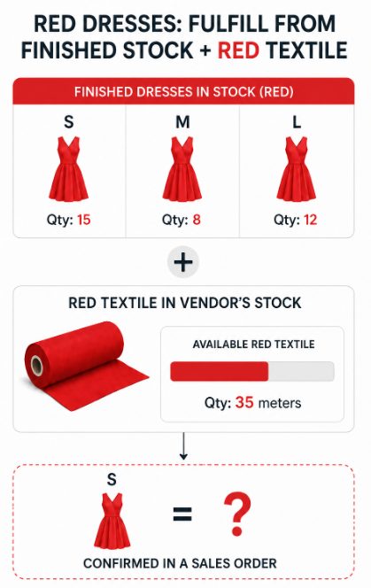
15 finished items in size S are in the warehouse.
35 metres of the shared material are at the supplier.
An order for size S arrives. How much can you confirm?
The correct answer needs two steps. First subtract what you already own. Then ask what the material can still cover – knowing that the same material also feeds M, L and every other variant in the range.
So the answer depends on what every other order promises in the same period.
This is not a fashion problem.
Replace the textile with a shared aluminium profile, a common casting, a coating line, a chip, or a contracted vendor capacity. The picture is identical: one constrained input feeding many finished products, while finished goods for some of those products already sit in the warehouse.
What usually happens
Either the promise ignores the constrained input and over-commits, or it consumes the constraint on every order line separately – and several orders quietly commit the same material twice.
What should happen
The two layers are consumed in a defined order, chosen by the business for that type of demand – and the shared input is committed once, not once per order line.
Starting point
What S/4HANA already does well.
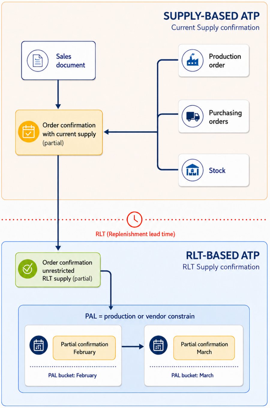
Advanced ATP separates the promise into two horizons, divided by the replenishment lead time. Inside the RLT, confirmation uses concrete supply. Beyond it, confirmation uses planned capacity expressed as product allocation.
Inside the lead time: real supply
Stock, purchase orders and production orders are concrete. The check confirms what physically exists or is firmly on its way.
Beyond the lead time: planned capacity
Nothing concrete exists yet, so the promise is made against a limit instead. Product allocation buckets represent what production or the vendor can deliver in a given period – at whatever level the constraint really lives: a component, a capacity group, a contract, a material family.
Both mechanisms are sound
Used on their own, each does exactly what it should. The difficulty is not in either half. It is in the seam between them.
The gap
Where the clean picture breaks.
In real order books the boundary is not a wall, and the two horizons are not independent. Four situations account for most of the damage.
Stock is never netted first
An order requested beyond the RLT consumes allocation capacity even when finished goods for that exact variant are standing in the warehouse. Capacity is spent on demand that was already covered, and the stock keeps ageing.
The boundary moves
Replenishment lead time is calculated, not fixed. Sourcing changes, component lead times, plant differences and calendar effects shift the boundary – so the same order can fall on different sides of it on different days.
Distant orders still need stock
A pre-order or frame call-off requested well beyond the RLT may still be intended to consume standing stock – especially at the end of a programme or season, when the commercial goal is to clear inventory rather than trigger new production.
The same supply counted twice
Physical stock and allocation capacity are two different axes. Correcting one without the other means the same supply is counted twice – or, after a naive fix, not at all.
The symptom on the shop floor
Confirmations look correct on the day they are given. The cost appears one or two quarters later, as ageing finished goods next to an order that could not be confirmed because capacity was already “used” – on goods that were sitting in the warehouse the whole time.
SizeGrid solution
Shared Constraint Availability.
A custom process built on standard aATP foundations. It uses the well-known RLT principle and extends it with product allocation, so that the two horizons stop working against each other. Which layer a given order consumes, and in which order, becomes a business rule instead of a side effect.
Establish the net picture
Before allocation is touched, determine what existing and committed supply can already cover for the requested variant and date.
- Works on the level where the constraint really lives
- Respects segmentation, plant and channel rules
- No virtual stock split, no shadow storage locations
Apply the configured sequence
Confirmation draws on the first layer up to the configured limit. Only the uncovered remainder continues to the second. Which layer comes first is a rule, set per type of demand.
- Stock first, or flexible capacity first – by scenario
- Protected quantities can be excluded from netting
- The netting horizon is a parameter, not a hard-coded rule
Cover the remainder from the second layer
The second layer is consumed only for the quantity the first could not cover, and only once – across all orders competing for the same constrained input.
- Prevents the same supply counting on both axes
- Keeps allocation buckets meaningful for planning
- Partial confirmation across periods stays intact
Behave the same way everywhere
The same logic applies in the online check, in backorder processing, in rescheduling and at delivery creation. A promise that only holds in one transaction is not a promise.
- Consistent result across all check contexts
- Traceable: every confirmation can be explained
- Built as an add-on, without modifying the SAP core
Configuration, not code
Both directions are legitimate.
There is no single correct sequence for every business, and a solution that hard-codes one is only half useful. What matters is that the choice is made deliberately, per type of demand, instead of falling out of how the check happens to be built.
Stock first, then capacity
Use what is already produced before committing new capacity against it. Right when the goal is to clear inventory: end of a programme, end of a season, ageing finished goods, or any range where the constrained input is scarcer than the warehouse.
Flexible capacity first, then stock
Send distant pre-orders to future capacity and only fall back on the warehouse if capacity runs out. This protects sellable stock for customers who want to buy now – near-term revenue is not given away to an order that will not ship for months.
The second case is the one most often missed. A pre-order booked far in advance looks harmless, but if it consumes standing stock, it quietly removes that stock from this month’s order book. The customer waiting until next season is served ahead of the customer buying today.
Shared Constraint Availability treats all of this as a rule set rather than a fixed behaviour: which demand consumes which layer, in which order, over which horizon, with which quantities protected, at which aggregation level. Commercial policy can change without a development cycle.
Netting horizon
How far into the future an order is still allowed to consume standing stock.
Protected quantities
Stock reserved for a channel, market or customer stays out of the netting.
Scope by hierarchy
Applied per product group, programme, market or capacity bucket – not globally.
Direction of the rule
Stock first or capacity first, decided per demand type instead of once for the whole system.
Business value
What changes in the order book.
Less ageing stock
Goods already produced are offered before new capacity is committed, so inventory turns instead of sitting through the next cycle.
More confirmable demand
Capacity that was silently consumed by already-covered orders becomes available for orders that genuinely need it.
Allocation stays meaningful
Buckets reflect real remaining capacity, so planners can trust the numbers they are steering with.
Aggregate flexibility survives
No need to break the constraint down to the lowest SKU level just to make the check behave – the reason allocation was introduced in the first place.
Fewer manual corrections
Customer service stops re-working confirmations in spreadsheets to compensate for what the check did automatically.
Today’s customers come first
Distant pre-orders can be pointed at future capacity, so stock on hand stays available for demand that ships this month.
Explainable promises
Each confirmation can be traced to the supply and capacity it consumed, which matters when a customer asks why the date moved.
Where it fits
Three conditions make this worth solving.
Where all three are true, the effect is usually visible within one planning cycle.
Orders arrive beyond the lead time
Pre-order programmes, project pipelines, frame contracts or campaign business, where a meaningful share of the order book is requested further out than production can react.
Capacity is managed at an aggregate level
The constraint is a component, a line, a vendor contract or a material family – deliberately kept above SKU level so the variant mix can stay flexible.
Standing stock is significant
Finished goods are regularly available that should be sold before new production capacity is committed against them.
Questions
Frequently asked questions.
Is this a replacement for standard aATP?
Do we have to redesign our product allocation objects?
Does it require modifications to the SAP core?
Should stock always be consumed before capacity?
What happens in backorder processing and rescheduling?
Can we test it on a limited scope first?
Our lead times are not stable. Does that break it?
Start with one product family.
Bring an order book where confirmations look right and stock keeps ageing anyway. We can show what the current check is doing with your own data, and what changes when existing supply is consumed first.
Discuss a pilot